GTMcore module¶

This module implements the generalized 4x4 transfer matrix (GTM) method poposed in Passler, N. C. and Paarmann, A., JOSA B 34, 2128 (2017) and corrected in JOSA B 36, 3246 (2019), as well as the layer-resolved absorption proposed in Passler, Jeannin and Paarman. This code uses inputs from D. Dietze’s FSRStools library https://github.com/ddietze/FSRStools

Please cite the relevant associated publications if you use this code.

Author:

Mathieu Jeannin mathieu.jeannin@c2n.upsaclay.fr math.jeannin@free.fr (permanent)

Affiliations:

Laboratoire de Physique de l’Ecole Normale Superieure (2019)
Centre de Nanosciences et Nanotechnologies (2020-2021)

Layers are represented by the Layer class that holds all parameters describing the optical properties of a single layer. The optical system is assembled using the System class.

Change log:

15-10-2021:

Fixed rounding error bug in lag.eig() causing the program to crash randomly

for negligibly small imaginary parts of the wavevectors

Corrected a sign error in gamma32 that lead to field discontinuities

19-03-2020:

Adapted the code to compute the layer-resolved absorption as proposed by Passler et al. (https://arxiv.org/abs/2002.03832), using System.calculate_Poynting_Absorption_vs_z().

Include the correct calculation of intensity transmission coefficients in System.calculate_r_t(). This BREAKS compatibility with the previous definition of the function.

Corrected bugs in System.calculate_Efield() and added magnetic field option

Adapted System.calculate_Efield() to allow hand-defined, irregular grid and a shorthand to compute only at layers interfaces. Regular grid with fixed resolution is left as an option.

20-09-2019:

Added functions in the System class to compute in-plane wavevector of guided modes and dispersion relation for such guided surface modes. This is highly prospective as it depends on the robustness of the minimization procedure (or the lack of thereoff)

The main algorithm is based on solving the eigenvalue equation for the electric field in each layer. The results are then propagated in a step-wised manner layer by layer accross the entire stack.

The Layer class¶

class GTM.GTMcore.Layer(thickness=1e-06, epsilon1=None, epsilon2=None, epsilon3=None, theta=0, phi=0, psi=0)¶

Layer class. An instance is a single layer:

thickness¶

thickness of the layer in m

Type: float

epsilon1¶

function epsilon(frequency) for the first axis. If none, defaults to vacuum.

Type: complex function

epsilon2¶

function epsilon(frequency) for the second axis. If none, defaults to epsilon1.

Type: complex function

epsilon3¶

function epsilon(frequency) for the third axis. If none, defaults to epsilon1.

Type: complex function

theta¶

Euler angle theta (colatitude) in rad

Type: float

phi¶

Euler angle phi in rad

Type: float

psi¶

Euler angle psi in rad

Type: float

Notes

If instanciated with defaults values, it generates a 1um thick layer of air. Properties can be checked/changed dynamically using the corresponding get/set methods.

set_thickness(thickness)¶

Sets the layer thickness

Parameters: thickness (float) – the layer thickness (in m)
Return type: None

set_epsilon(epsilon1=<function vacuum_eps>, epsilon2=None, epsilon3=None)¶

Sets the dielectric functions for the three main axis.

Parameters

epsilon1 (func) – function epsilon(frequency) for the first axis. If none, defaults to vacuum_eps()
epsilon2 (complex function) – function epsilon(frequency) for the second axis. If none, defaults to epsilon1.
epsilon3 (complex function) – function epsilon(frequency) for the third axis. If none, defaults to epsilon1.
epsilon1 –

Return type

None

Notes

Each epsilon_i function returns the dielectric constant along axis i as a function of the frequency f in Hz.

If no function is given for epsilon1, it defaults to vacuum_eps() (1.0 everywhere). epsilon2 and epsilon3 default to epsilon1: if None, a homogeneous material is assumed

calculate_epsilon(f)¶

Sets the value of epsilon in the (rotated) lab frame.

Parameters: f (float) – frequency (in Hz)
Return type: None

Notes

The values are set according to the epsilon_fi (i=1..3) functions defined using the set_epsilon() method, at the given frequency f. The rotation with respect to the lab frame is computed using the Euler angles.

Use only explicitely if you don’t use the Layer.update() function!

set_euler(theta, phi, psi)¶

Sets the values for the Euler rotations angles.

Parameters

theta (float) – Euler angle theta (colatitude) in rad
phi (float) – Euler angle phi in rad
psi (float) – Euler angle psi in rad

Return type

None

calculate_matrices(zeta)¶

Calculate the principal matrices necessary for the GTM algorithm.

Parameters: zeta (complex) – In-plane reduced wavevector kx/k0 in the system.
Return type: None

Notes

Note that zeta is conserved through the whole system and set externaly using the angle of incidence and System.superstrate.epsilon[0,0] value

Requires prior execution of calculate_epsilon()

calculate_q()¶

Calculates the 4 out-of-plane wavevectors for the current layer.

Return type: None

Notes

From this we also get the Poynting vectors. Wavevectors are sorted according to (trans-p, trans-s, refl-p, refl-s) Birefringence is determined according to a threshold value qsd_thr set at the beginning of the script.

calculate_gamma(zeta)¶

Calculate the gamma matrix

Parameters: zeta (complex) – in-plane reduced wavevector kx/k0
Return type: None

calculate_transfer_matrix(f, zeta)¶

Compute the transfer matrix of the whole layer \(T_i=A_iP_iA_i^{-1}\)

Parameters

f (float) – frequency (in Hz)
zeta (complex) – reduced in-plane wavevector kx/k0

Return type

None

update(f, zeta)¶

Shortcut to recalculate all layer properties.

Parameters

f (float) – frequency (in Hz)
zeta (complex) – reduced in-plane wavevector kx/k0

Returns

Ai (4x4-array) – Boundary matrix \(A_i\) of the layer
Ki (4x4-array) – Propagation matrix \(K_i\) of the layer
Ai_inv (4x4-array) – Inverse of the \(A_i\) matrix
Ti (4x4-array) – Transfer matrix of the whole layer

The System class¶

class GTM.GTMcore.System(substrate=None, superstrate=None, layers=[])¶

System class. An instance is an optical system with substrate, superstrate and layers.

theta¶

Angle of incidence, in radians

Type: float

substrate¶

The substrate layer. Defaults to vacuum (empty layer instance)

Type: Layer

superstrate¶

The superstrate layer, defaults to vacuum (empty layer instance)

Type: Layer

layers¶

list of the layers in the system

Type: list of layers

Notes

Layers can be added and removed (not inserted).

The whole system’s transfer matrix is computed using calculate_GammaStar(), which calls Layer.update() for each layer. General reflection and transmission coefficient functions are given, they require prior execution of calculate_GammaStar(). The electric fields can be visualized in the case of incident plane wave using calculate_Efield()

set_substrate(sub)¶

Sets the substrate

Parameters: sub (Layer) – Instance of the layer class, substrate
Return type: None

set_superstrate(sup)¶

Set the superstrate

Parameters: sup (Layer) – Instance of the layer class, superstrate
Return type: None

get_all_layers()¶

Returns the list of all layers in the system

Returns: l – list of all layers
Return type: list

get_layer(pos)¶

Get the layer at a given position

Parameters: pos (int) – position in the stack
Returns: L – The layer at the position pos
Return type: Layer

get_superstrate()¶

Returns the System’s superstrate

Returns: L – The system superstrate
Return type: Layer

get_substrate()¶

Returns the System’s substrate

Returns: L – The system substrate
Return type: Layer

add_layer(layer)¶

Add a layer instance.

Parameters: layer (Layer) – The layer to be added on the stack
Return type: None

Notes

The layers are added from superstrate to substrate order. Light is incident from the superstrate.

Note thate this function adds a reference to L to the list. If you are adding the same layer several times, be aware that if you change something for one of them, it changes all of them.

del_layer(pos)¶

Remove a layer at given position. Does nothing for invalid position.

Parameters: pos (int) – Index of layer to be removed.
Return type: None

initialize_sys(f)¶

Sets the values of epsilon at the given frequency in all the layers.

Parameters: f (float) – Frequency (Hz)
Return type: None

Notes

This function allows to define the in-plane wavevector (\(zeta\)) outside of the class, and thus to explore also guided modes of the system.

calculate_GammaStar(f, zeta_sys)¶

Calculate the whole system’s transfer matrix.

Parameters

f (float) – Frequency (Hz)
zeta_sys (complex) – In-plane wavevector kx/k0

Returns

GammaStar – System transfer matrix \(\Gamma^{*}\)

Return type

4x4 complex matrix

calculate_r_t(zeta_sys)¶

Calculate various field and intensity reflection and transmission coefficients, as well as the 4-valued vector of transmitted field.

Parameters

zeta_sys (complex) – Incident in-plane wavevector

Returns

r_out (len(4)-array) – Complex field reflection coefficients r_out=([rpp,rps,rss,rsp])
R_out (len(4)-array) – Real intensity reflection coefficients R_out=([Rpp,Rss,Rsp,Tps])
t_out (len(4)-array) – Complex field transmition coefficients t=([tpp, tps, tsp, tss])
T_out (len(4)-array) – Real intensity transmition coefficients T_out=([Tp,Ts]) (mode-inselective)

Notes

IMPORTANT ..version 19-03-2020: All intensity coefficients are now well defined. Transmission is defined mode-independently. It could be defined mode-dependently for non-birefringent substrates in future versions. The new definition of this function BREAKS compatibility with the previous one.

..version 13-09-2019: Note that the field reflectivity and transmission coefficients r and t are well defined. The intensity reflection coefficient is also correct. However, the intensity transmission coefficients T are ill-defined so far. This will be corrected upon future publication of the correct intensity coefficients.

Note also the different ordering of the coefficients, for consistency w/ Passler’s matlab code

calculate_Efield(f, zeta_sys, z_vect=None, x=0.0, magnetic=False, dz=None)¶

Calculate the electric field profiles for both s-pol and p-pol excitation.

Parameters

f (float) – frequency (Hz)
zeta_sys (complex) – in-plane normalized wavevector kx/k0
z_vect (1Darray) – Coordinates at which the calculation is done. if None, the layers boundaries are used.
x (float or 1D array) – x-coordinates for (future) 2D plot of the electric field. Not yet implemented
magnetic (bool) – Boolean to skip or compute the magnetic field vector
dz (float (optional)) – Space resolution along propagation (z) axis. Superseed z_vect

Returns

z (1Darray) – 1D array of z-coordinates according to dz
E_out ((len(z),3)-Array) – Total electric field in the structure
H_out (opt) ((len(z),3)-Array) – Total magnetic field in the structure
zn (list) – Positions of the different interfaces

Notes

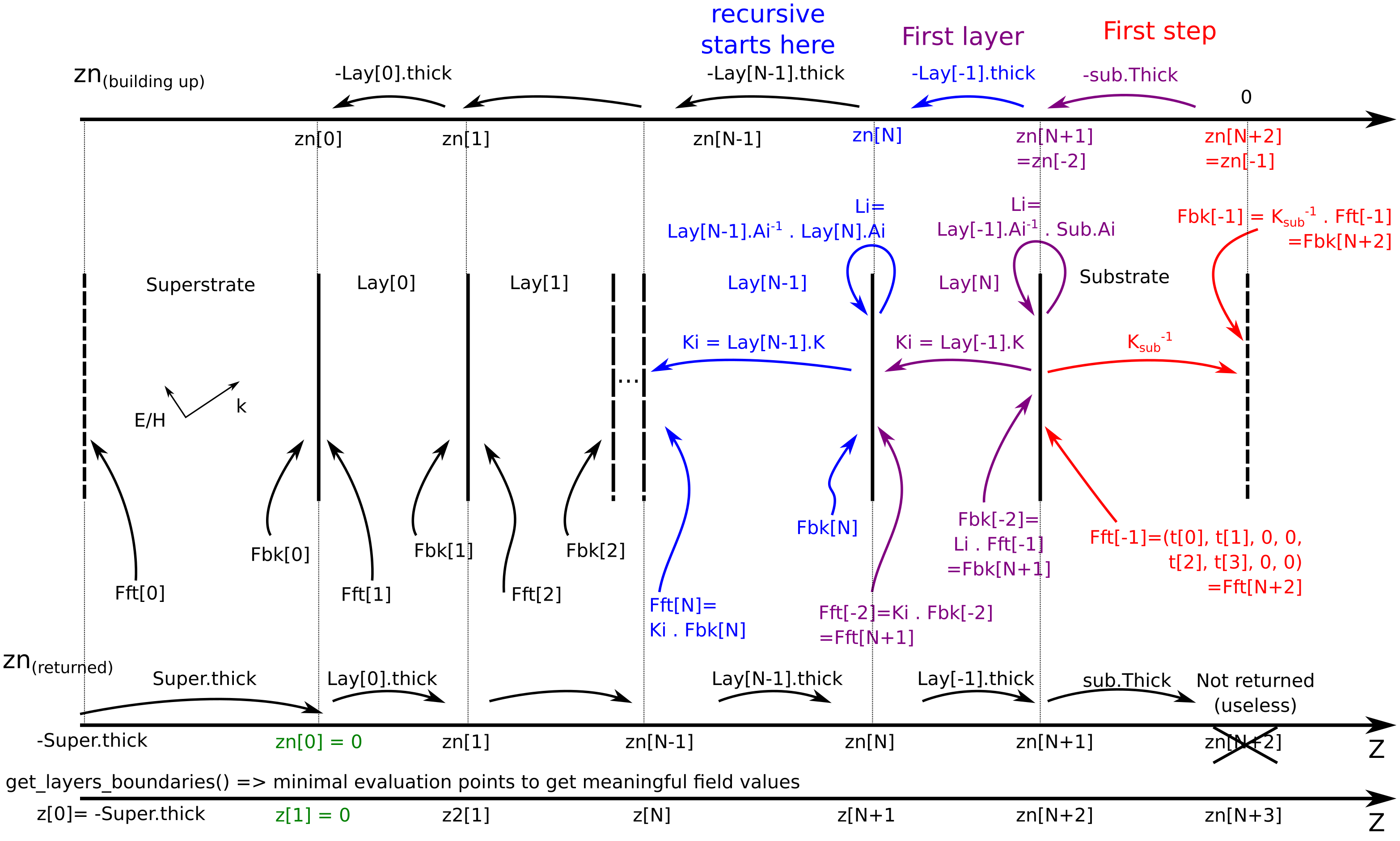
..Version 19-03-2020:: changed keywords to add z_vect z_vect is used for either minimal computation (using get_layers_boundaries) or hand-defined z-positions (e.g. irregular spacing for improved resolution) if dz is given, a regular grid is used. A sketch of the definition of all fields and algorithm is supplied in the module, to better get a grasp on where Fft and Fbk are defined.
..Version 28-01-2020:: Added Magnetic field keyword to save time. Poyting and absorption defined in a separate function
..Version 06-01-2020:: Added Magnetic field and Poyting vector.
..Version 13-09-2019:: the 2D field profile is not implemented yet. x should be left to default

calculate_Poynting_Absorption_vs_z(z, E, H, R)¶

Calculate the z-dependent Poynting vector and cumulated absorption.

Parameters

z (1Darray) – Spatial coordinate for the fields
E (1Darray) – 6-components Electric field vector (p- or s- in) along z
H (1Darray) – 6-components Magnetic field vector (p- or s- in) along z
R (len(4)-array) – Reflectivity from calculate_r_t()
S_out (6xlen(z) array) – 6 components (p//s) Poyting vector along z
A_out (2xlen(z)) – 2 components (p//s) absorption along z

get_layers_boundaries()¶

Return the z-position of all boundaries, including the “top” of the superstrate and the “bottom” of the substrate. This corresponds to where the fields should be evaluated to get a minimum of information

Returns: zn – Array of layer boundary positions
Return type: 1Darray

get_spatial_permittivity(z)¶

Extract the permittivity tensor at given z in the structure

Parameters: z (1Darray) – Array of points to sample the permittivity
Returns: eps – Complex permittivity tensor as a function of z
Return type: 3x3xlen(z)-array

calculate_matelem(zeta0, f)¶

Calculate the common denominator of all reflexion/transmission coefficients.

Parameters

zeta0 (2-tuple) – Tuple [zeta_r, zeta_i] of real and imaginary part of the wavevector
f (float) – frequency (in Hz)

Returns

matelem – Matrix element to minimize for dispersion relation (absolute value)

Return type

complex

Notes

Returns the relevant quantity to find waveguide modes according to Davis’ paper on multilayers (scalar model http://doi.org/10.1016/j.optcom.2008.09.043) and then Yeh (4X4 formalism http://doi.org/10.1016/0039-6028(80)90293-9).

calculate_eigen_wv(zeta0, f, bounds=None)¶

Calculate the eigenmode in-plane wavevector that shows guiding along the plane.

Parameters

zeta0 (2-tuple) – Initial guess for the minimization procedure
f (float) – Frequency (in Hz)
bounds (list (optional)) – list of 2-tuple containing (lower, upper) bound for each parameter

Returns

res – Result of the minimization procedure. Eigenvalue is the list res.x

Return type

OptimizeResult

Notes

Based on the idea that guided mode := an output field exists with no input field This is strongly dependant on the minimization procedure and thus has to be consistently and carefully checked.

disp_vs_f(fv, zeta0, bounds=None)¶

Performs a frequency dependent search of the eigenwavevector for a guided mode to get the dispersion relation of a surface mode.

Provided a reasonable initial guess for the first frequency point, we use the eigen_wv from the above method and follow its value as a function of frequency in a stepping manner.

Parameters

fv (1Darray) – Array of frequencies
zeta0 (2-tuple) – Initial guess for the minimization
bounds (list) – list of 2-tuple containing (lower, upper) bound for each parameter

Returns

zeta_disp_r (1Darray (complex)) – Array of real part of the in-plane wavevector
zeta_disp_i (1Darray (complex)) – Array of imaginary part of the in-plane wavevector

Additional functions¶

GTM.GTMcore.exact_inv(M)¶

Compute the ‘exact’ inverse of a 4x4 matrix using the analytical result.

Parameters: M (4X4 array (float or complex)) – Matrix to be inverted
Returns: out – Inverse of this matrix or Moore-Penrose approximation if matrix cannot be inverted.
Return type: 4X4 array (complex)

Notes

This should give a higher precision and speed at a reduced noise. From D.Dietze code https://github.com/ddietze/FSRStools

pyGTM

Navigation

Related Topics

GTMcore module¶

The Layer class¶

The System class¶

Additional functions¶